Overview of capabilities
Main features
- Newton-Krylov solver with generic linear / eigen preconditioned solver. Idem for the arc-length continuation.
- Newton-Krylov solver with nonlinear deflation and preconditioner. It can be used for branch switching for example. It is used for deflated continuation.
- Continuation written as an Iterator Interface.
- Monitoring user functions along curves computed by continuation, see Event Handling.
- Continuation methods: PALC, Moore Penrose, Multiple, Polynomial, Deflated continuation, ANM, ...
- Bifurcation points / events located with bisection.
- Compatible with GPU
Capabilities related to equilibria
- Detection of Branch, Fold, Hopf bifurcation points of stationary solutions and computation of their normal form. Other non-generic bifurcations based on spectrum are also detected.
- Automatic branch switching at branch points (whatever the dimension of the kernel) to equilibria
- Automatic computation of bifurcation diagrams of equilibria
- Fold / Hopf continuation based on Minimally Augmented formulation, with Matrix Free / Sparse / Dense Jacobian.
- Detection of all codim 2 bifurcations of equilibria and computation of the normal forms of Bogdanov-Takens, Bautin, Cusp, Zero-Hopf and Hopf-Hopf.
- Branching from Bogdanov-Takens / Zero-Hopf / Hopf-Hopf points to Fold / Hopf curve
(limited) Capabilities related to maps
- continuation of fixed points of maps
- computation of normal form of Period-doubling, Neimark-Sacker, Branch point bifurcations.
Summary table for equilibria
Note that you can combine most solvers, like use Deflation for Periodic orbit computation or Fold of periodic orbits family.
Custom state means, you can use something else than
AbstractArray, for example your ownstruct.
| Features | Matrix Free | Custom state | Tutorial | GPU |
|---|---|---|---|---|
| (Deflated) Krylov-Newton | Yes | Yes | Deflated problems | Yes |
| Continuation PALC (Natural, Secant, Tangent, Polynomial) | Yes | Yes | All | Yes |
| Deflated Continuation | Yes | Yes | Deflated continuation in the Carrier problem | Yes |
| Bifurcation / Fold / Hopf point detection | Yes | Yes | All | Yes |
| Fold Point continuation | Yes | Yes | Temperature model (codim 2), 2d Ginzburg-Landau equation (finite differences, codim 2, Hopf aBS), Extended Lorenz-84 model (codim 2 + BT/ZH aBS) | Yes |
| Hopf Point continuation | Yes | AbstractArray | Extended Lorenz-84 model (codim 2 + BT/ZH aBS) | |
| Branch point / Fold / Hopf normal form | Yes | Yes | 1d Brusselator (automatic) | |
| Branch switching at Branch points | Yes | AbstractArray | From simple branch point to equilibria | Yes |
| Automatic bifurcation diagram computation of equilibria | Yes | AbstractArray | pp2 example from AUTO07p (aBD + Hopf aBS) | |
| Bogdanov-Takens / Bautin / Cusp / Zero-Hopf / Hopf-Hopf point detection | Yes | Yes | Extended Lorenz-84 model (codim 2 + BT/ZH aBS) | |
| Bogdanov-Takens / Bautin / Cusp normal forms | Yes | AbstractArray | Extended Lorenz-84 model (codim 2 + BT/ZH aBS) | Yes |
| Branching from Bogdanov-Takens / Zero-Hopf / Hopf-Hopf to Fold / Hopf curve | Yes | AbstractArray | Extended Lorenz-84 model (codim 2 + BT/ZH aBS) |
Capabilities related to Periodic orbits (PO)
- PO computation and continuation using parallel (Standard or Poincaré) Shooting, Finite Differences or Orthogonal Collocation (mesh adaptive).
- Automatic branch switching from simple Hopf points to PO
- Automatic branch switching from simple Period-Doubling points to PO
- Assisted branch switching from simple Branch points to PO
- Detection of Branch, Fold, Neimark-Sacker (NS), Period Doubling (PD) bifurcation points of PO.
- Fold / PD / NS continuation based on Minimally Augmented formulation (for shooting and collocation). Trapezoid method only allows continuing Fold of PO.
- Detection of all codim 2 bifurcations of PO (R1, R2, R3, R4, GPD, NS-NS, Chenciner, Fold-Flip, Fold-NS, PD-NS)
- Computation of the normal forms of PD, NS (for shooting and collocation) using the method based on Poincaré return map or the Iooss normal form.
- automatic branching from Bautin to curve of Fold of PO
- automatic branching from Zero-Hopf to curve of NS of PO
- automatic branching from Hopf-Hopf to curve of NS of PO
Legend for the table: Standard shooting (SS), Poincaré shooting (PS), Orthogonal collocation (OC), trapezoid (T).
| Features | Method | Matrix Free | Custom state | Tutorial | GPU |
|---|---|---|---|---|---|
| Branch switching at Hopf points | SS/PS/OC/T | See each | Neural mass equation (Hopf aBS) | ||
| Newton / continuation | T | Yes | AbstractVector | 1d Brusselator (automatic), 2d Ginzburg-Landau equation (finite differences, codim 2, Hopf aBS) | Yes |
| Newton / continuation | OC | AbstractVector | Neural mass equation (Hopf aBS) | ||
| Newton / continuation | SS | Yes | AbstractArray | Period doubling in Lur'e problem (PD aBS) | Yes |
| Newton / continuation | PS | Yes | AbstractArray | 1d Brusselator (automatic) | Yes |
| Fold, Neimark-Sacker, Period doubling detection | SS/PS/OC/T | See each | AbstractVector | 1d Brusselator (automatic) | |
| Branch switching at Branch point | SS/PS/OC/T | See each | Period doubling in Lur'e problem (PD aBS) | ||
| Branch switching at PD point | SS/PS/OC/T | See each | Period doubling in Lur'e problem (PD aBS) | ||
| Continuation of Fold points | SS/PS/OC/T | See each | AbstractVector | Periodic predator-prey model 2d Ginzburg-Landau equation (finite differences, codim 2, Hopf aBS) | Yes |
| Continuation of Period-doubling points | SS/OC | AbstractVector | Periodic predator-prey model | ||
| Continuation of Neimark-Sacker points | SS/OC | AbstractVector | Steinmetz-Larter model | ||
| detection of codim 2 bifurcations of periodic orbits | SS/OC | AbstractVector | Steinmetz-Larter model | ||
| Branch switching at Bautin point to curve of Fold of periodic orbits | SS/OC | AbstractVector | Lorenz-84 model, take 2 | ||
| Branch switching at ZH/HH point to curve of NS of periodic orbits | SS/OC | AbstractVector | Lorenz-84 model, take 2 |
Capabilities related to Homoclinic orbits
These are available through the plugin HclinicBifurcationKit.jl. Please see the specific docs for more information.
- compute Homoclinic to Hyperbolic Saddle Orbits (HomHS) using Orthogonal collocation or Standard shooting
- compute bifurcation of HomHS
- start HomHS from a direct simulation
- automatic branch switching to HomHS from Bogdanov-Takes bifurcation point
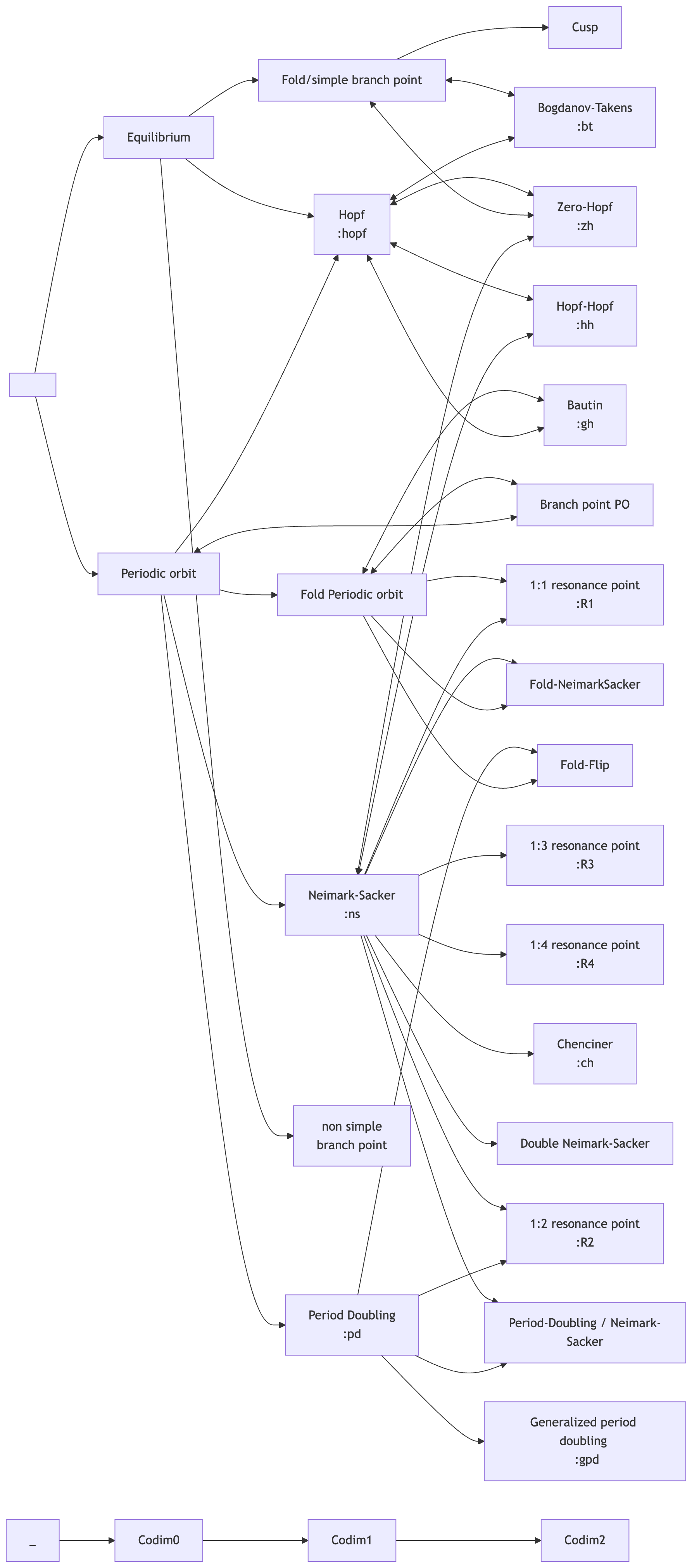
List of detected bifurcations
A left-to-right arrow in the following graph from $E_1$ to $E_2$ means that $E_2$ can be detected when continuing an object of type $E_1$.
A right-to-left arrow from $E_2$ to $E_1$ means that we can start the computation of object of type $E_1$ from $E_2$.
Each object of codim 0 (resp. 1) can be continued with 1 (resp. 2) parameters.