Deflated Continuation

Deflated continuation allows to compute branches of solutions to the equation $F(x,p)=0$. It is based on the Deflated Newton (see Deflated problems) algorithm.

See DefCont for more information.

However, unlike the regular continuation method, deflated continuation allows to compute disconnected bifurcation diagrams, something that is impossible for our Automatic Bifurcation diagram computation which is limited to the connected component of the initial point.

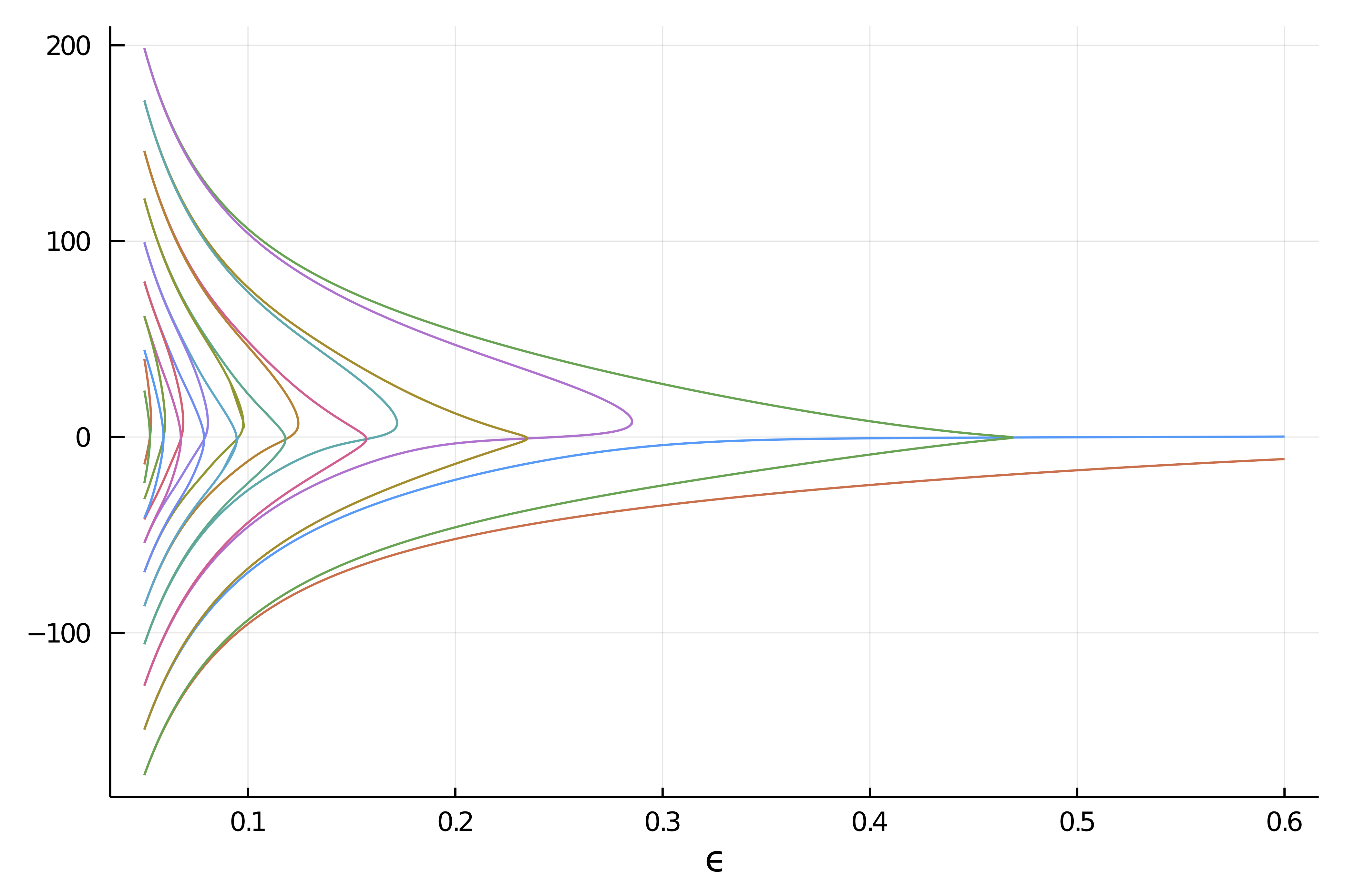
You can find an example of use of the method in Carrier Problem. We reproduce below the result of the computation which shows various disconnected components arising form Fold bifurcations that are found seemingly by the method.

Algorithm

Input: Initial parameter value λmin.
Input: Final parameter value λmax > λmin. Input: Step size ∆λ > 0.
Input: Nonlinear residual f(u,λ).
Input: Deflation operator M(u; u∗).
Input: Initial solutions S(λmin) to f(·,λmin).
λ ← λmin
while λ < λmax do
	F(·) ← f(·,λ+∆λ) 						# Fix the value of λ to solve for.
	S(λ+∆λ) ← ∅
	for u0 ∈ S(λ) do 						# Continue known branches.
		apply Newton’s method to F from initial guess u0.
		if solution u∗ found then
			S(λ + ∆λ) ← S(λ + ∆λ) ∪ {u∗}  # Record success
			F(·) ← M(·;u∗)F(·)			  # Deflate solution

	for u0 ∈ S(λ) do 					  # Seek new branches.
		success ← true
		while success do
			apply Newton’s method to F from initial guess u0.
			if solution u∗ found then		 # New branch found
				S(λ + ∆λ) ← S(λ + ∆λ) ∪ {u∗} # Record success
				F(·) ← M(·;u∗)F(·)		     # Deflate solution
		else
			success ← false
	λ←λ+∆λ
return S

Tips

The following piece of information is valuable in order to get the algorithm working in various conditions (see also here) especially for small systems (e.g. dim<20):

• newton is quite good and it is convenient to limit it otherwise it will be able to bypass the deflation. For example, you can use maxIter = 10 in NewtonPar
• try to limit the newton residual by using the argument callback_newton = BifurcationKit.cbMaxNorm(1e7). This will likely remove the occurrence of ┌ Error: Same solution found for identical parameter value!!
• finally, you can try some aggressive shift (here 0.01 in the deflation operator, like DeflationOperator(2, dot, 0.01, [sol]) but use it wisely.

Basic example

We show a quick and simple example of use. Note in particular that the algorithm is able to find the disconnected branch. The starting points are marked with crosses

using BifurcationKit, LinearAlgebra, Setfield, SparseArrays, Plots
const BK = BifurcationKit

k = 2
N = 1
F(x, p) = @. p * x + x^(k+1)/(k+1) + 0.01
Jac_m(x, p) = diagm(0 => p .+ x.^k)

# bifurcation problem
prob = BifurcationProblem(F, [0.], 0.5, (@lens _), J = Jac_m)

# continuation options
opts = BK.ContinuationPar(dsmax = 0.051, dsmin = 1e-3, ds=0.001, max_steps = 140, p_min = -3., newton_options = NewtonPar(tol = 1e-8), save_eigenvectors = false)

# algorithm
alg = BK.DefCont(deflation_operator = DeflationOperator(2, .001, [[0.]]), perturb_solution = (x,p,id) -> (x  .+ 0.1 .* rand(length(x))))

brdc = continuation(prob, alg,
	ContinuationPar(opts, ds = -0.001, max_steps = 800, newton_options = NewtonPar(verbose = false, max_iterations = 6), plot_every_step = 40),
	; plot=true, verbosity = 0,
	callback_newton = BK.cbMaxNorm(1e3) # reject newton step if residual too large
	)
plot(brdc)