🟡 Colpitts–type Oscillator

• 🟡 Colpitts–type Oscillator
• • Periodic orbits with Multiple Standard Shooting
  • References

In this tutorial, we show how to study parametrized quasilinear DAEs like:

\[A(\mu,x)\dot x = G(\mu,x).\]

In particular, we detect a Hopf bifurcation and compute the periodic orbit branching from it using a multiple standard method.

The following DAE model is taken from ^[Rabier]:

\[\left(\begin{array}{cccc} -\left(C_{1}+C_{2}\right) & C_{2} & 0 & 0 \\ C_{2} & -C_{2} & 0 & 0 \\ C_{1} & 0 & 0 & 0 \\ 0 & 0 & L & 0 \end{array}\right)\left(\begin{array}{c} \dot{x}_{1} \\ \dot{x}_{2} \\ \dot{x}_{3} \\ \dot{x}_{4} \end{array}\right)=\left(\begin{array}{c} R^{-1}\left(x_{1}-V\right)+I E\left(x_{1}, x_{2}\right) \\ x_{3}+I C\left(x_{1}, x_{2}\right) \\ -x_{3}-x_{4} \\ -\mu+x_{2} \end{array}\right)\]

It is easy to encode the DAE as follows. The mass matrix is defined next.

using Revise, Parameters, Plots
using BifurcationKit
using LinearAlgebra # for eigen
const BK = BifurcationKit

# function to record information from the soluton
recordFromSolution(x, p) = (u1 = norminf(x), x1 = x[1], x2 = x[2], x3 = x[3], x4 = x[4])

# vector field
f(x, p) = p.Is * (exp(p.q * x) - 1)
IE(x1, x2, p) = -f(x2, p) + f(x1, p) / p.αF
IC(x1, x2, p) = f(x2, p)/ p.αR - f(x1, p)

function Colpitts!(dz, z, p, t = 0)
	@unpack C1, C2, L, R, Is, q, αF, αR, V, μ = p
	x1, x2, x3, x4 = z
	dz[1] = (x1 - V) / R + IE(x1, x2, p)
	dz[2] =	x3 + IC(x1, x2, p)
	dz[3] = -x3-x4
	dz[4] = -μ+x2
	dz
end

# parameter values
par_Colpitts = (C1 = 1.0, C2 = 1.0, L = 1.0, R = 1/4., Is = 1e-16, q = 40., αF = 0.99, αR = 0.5, μ = 0.5, V = 6.)

# initial condition
z0 = [0.9957,0.7650,19.81,-19.81]

# mass matrix
Be = [-(par_Colpitts.C1+par_Colpitts.C2) par_Colpitts.C2 0 0;par_Colpitts.C2 -par_Colpitts.C2 0 0;par_Colpitts.C1 0 0 0; 0 0 par_Colpitts.L 0]

# we group the differentials together
prob = BifurcationProblem(Colpitts!, z0, par_Colpitts, (@lens _.μ); record_from_solution = recordFromSolution)

We first compute the branch of equilibria. But we need a generalized eigenvalue solver for this.

# we need  a specific eigensolver with mass matrix B
struct EigenDAE{Tb} <: BK.AbstractDirectEigenSolver
	B::Tb
end

# compute the eigen elements
function (eig::EigenDAE)(Jac, nev; k...)
	F = eigen(Jac, eig.B)
	I = sortperm(F.values, by = real, rev = true)
	return Complex.(F.values[I]), Complex.(F.vectors[:, I]), true, 1
end

# continuation options
optn = NewtonPar(tol = 1e-13, max_iterations = 10, eigsolver = EigenDAE(Be))
opts_br = ContinuationPar(p_min = -0.4, p_max = 0.8, ds = 0.01, dsmax = 0.01, nev = 4, plot_every_step = 3, max_steps = 1000, newton_options = optn)
	opts_br = @set opts_br.newton_options.verbose = false
	br = continuation(prob, PALC(), opts_br; normC = norminf)

scene = plot(br, vars = (:param, :x1))

Periodic orbits with Multiple Standard Shooting

We use shooting to compute periodic orbits: we rely on a fixed point of the flow. To compute the flow, we use DifferentialEquations.jl.

Thanks to ^[Lamour], we can just compute the Floquet coefficients to get the nonlinear stability of the periodic orbit. Two period doubling bifurcations are detected.

Note that we use Automatic Branch Switching from a Hopf bifurcation despite the fact the normal form implemented in BifurcationKit.jl is not valid for DAE. For example, it predicts a subciritical Hopf point whereas we see below that it is supercritical. Nevertheless, it provides a

using DifferentialEquations

# this is the ODEProblem used with `DiffEqBase.solve`
# we  set  the initial conditions
prob_dae = ODEFunction(Colpitts!; mass_matrix = Be)
probFreez_ode = ODEProblem(prob_dae, z0, (0., 1.), par_Colpitts)

# we lower the tolerance of newton for the periodic orbits
optnpo = @set optn.tol = 1e-9
@set! optnpo.eigsolver = DefaultEig()

opts_po_cont = ContinuationPar(dsmin = 0.0001, dsmax = 0.005, ds= -0.0001, p_min = 0.2, max_steps = 50, newton_options = optnpo, nev = 4, tol_stability = 1e-3, plot_every_step = 5)


# Shooting functional. Note the  stringent tolerances used to cope with
# the extreme parameters of the model
probSH = ShootingProblem(10, probFreez_ode, Rodas5P(); reltol = 1e-10, abstol = 1e-13)

# automatic branching from the Hopf point
br_po = continuation(br, 1, opts_po_cont, probSH;
	plot = true, verbosity = 3,
	linear_algo = MatrixBLS(),
	# δp is use to parametrise the first parameter point on the
	# branch of periodic orbits
	δp = 0.001,
	record_from_solution = (u, p) -> begin
		outt = BK.get_periodic_orbit(p.prob, u, (@set  par_Colpitts.μ=p.p))
		m = maximum(outt[1,:])
		return (s = m, period = u[end])
	end,
	# plotting of a solution
	plot_solution = (x, p; k...) -> begin
		outt = BK.get_periodic_orbit(p.prob, x, (@set  par_Colpitts.μ=p.p))
		plot!(outt.t, outt[2,:], subplot = 3)
		plot!(br, vars = (:param, :x1), subplot = 1)
	end,
	# the newton Callback is used to reject residual > 1
	# this is to avoid numerical instabilities from DE.jl
	callback_newton = BK.cbMaxNorm(1.0),
	normC = norminf)

 ┌─ Curve type: PeriodicOrbitCont from Hopf bifurcation point.
 ├─ Number of points: 38
 ├─ Type of vectors: Vector{Float64}
 ├─ Parameter μ starts at 0.7642229295455085, ends at 0.6351258517235856
 ├─ Algo: PALC
 └─ Special points:

- #  1,       pd at μ ≈ +0.73090682 ∈ (+0.73090682, +0.73162733), |δp|=7e-04, [converged], δ = ( 1,  1), step =  17
- #  2,       pd at μ ≈ +0.67281695 ∈ (+0.67281695, +0.67355881), |δp|=7e-04, [converged], δ = (-1, -1), step =  27
- #  3, endpoint at μ ≈ +0.63512585,                                                                     step =  37

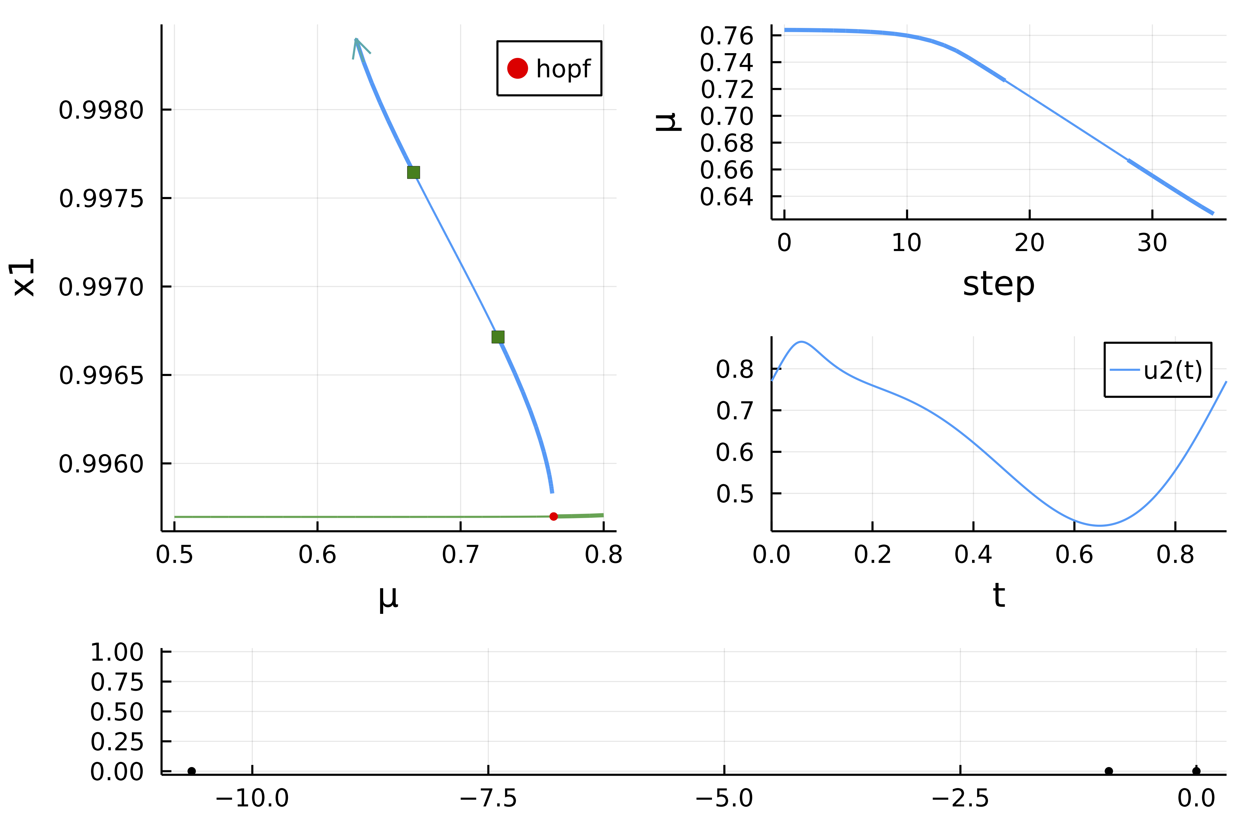
with detailed information

 ┌─ Curve type: PeriodicOrbitCont from Hopf bifurcation point.
 ├─ Number of points: 38
 ├─ Type of vectors: Vector{Float64}
 ├─ Parameter μ starts at 0.7642229295455086, ends at 0.6352549726782099
 ├─ Algo: PALC
 └─ Special points:

If `br` is the name of the branch,
ind_ev = index of the bifurcating eigenvalue e.g. `br.eig[idx].eigenvals[ind_ev]`

- #  1,       pd at μ ≈ +0.73116245 ∈ (+0.73116245, +0.73152250), |δp|=4e-04, [converged], δ = ( 1,  1), step =  17, eigenelements in eig[ 18], ind_ev =   1
- #  2,       pd at μ ≈ +0.67272920 ∈ (+0.67272920, +0.67310008), |δp|=4e-04, [converged], δ = (-1, -1), step =  27, eigenelements in eig[ 28], ind_ev =   1
- #  3, endpoint at μ ≈ +0.63525497,                                                                     step =  37

Let us show that this bifurcation diagram is valid by showing evidences for the period doubling bifurcation.

probFreez_ode = ODEProblem(prob_dae, br.specialpoint[1].x .+ 0.01rand(4), (0., 200.), @set par_Colpitts.μ = 0.733)

solFreez = @time solve(probFreez_ode, Rodas4(), progress = true;reltol = 1e-10, abstol = 1e-13)

scene = plot(solFreez, vars = [2], xlims=(195,200), title="μ = $(probFreez_ode.p.μ)")

and after the bifurcation

probFreez_ode = ODEProblem(prob_dae, br.specialpoint[1].x .+ 0.01rand(4), (0., 200.), @set par_Colpitts.μ = 0.72)

solFreez = @time solve(probFreez_ode, Rodas4(), progress = true;reltol = 1e-10, abstol = 1e-13)

scene = plot(solFreez, vars = [2], xlims=(195,200), title="μ = $(probFreez_ode.p.μ)")

References