🟡 2d Bratu–Gelfand problem with Gridap.jl

• 🟡 2d Bratu–Gelfand problem with Gridap.jl
• • Computation of the first branches

We re-consider the problem of Mittelmann treated in the previous tutorial but using a finite elements method (FEM) implemented in the package Gridap.jl.

Recall that the problem is defined by solving

\[\Delta u +NL(\lambda,u) = 0\]

with Neumann boundary condition on $\Omega = (0,1)^2$ and where $NL(\lambda,u)\equiv-10(u-\lambda e^u)$.

We start by installing the package GridapBifurcationKit.jl. Then, we can import the different packages:

using Revise
using Plots, Gridap, Setfield
using Gridap.FESpaces
using GridapBifurcationKit, BifurcationKit

# custom plot function to deal with Gridap
plotgridap!(x; k...) = (n=isqrt(length(x));heatmap!(reshape(x,n,n); color=:viridis, k...))
plotgridap(x; k...) =( plot();plotgridap!(x; k...))

We are now ready to specify the problem using the setting of Gridap.jl: it allows to write the equations very closely to the mathematical formulation:

# discretisation
n = 40
domain = (0, 1, 0, 1)
cells = (n,n)
model = CartesianDiscreteModel(domain,cells)

# function spaces
order = 1
reffe = ReferenceFE(lagrangian, Float64, order)
V = TestFESpace(model, reffe, conformity=:H1,)#dirichlet_tags="boundary")
U = TrialFESpace(V)

Ω = Triangulation(model)
degree = 2*order
const dΩ = Measure(Ω, degree) # we make it const because it is used in res

# nonlinearity
NL(u) = exp(u)

# residual
res(u,p,v) = ∫( -∇(v)⋅∇(u) -  v ⋅ (u - p.λ ⋅ (NL ∘ u)) * 10 )*dΩ

# jacobian of the residual
jac(u,p,du,v) = ∫( -∇(v)⋅∇(du) - v ⋅ du ⋅ (1 - p.λ * ( NL ∘ u)) * 10 )*dΩ

# 3rd and 4th derivatives, used for aBS
d2res(u,p,du1,du2,v) = ∫( v ⋅ du1 ⋅ du2 ⋅ (NL ∘ u) * 10 * p.λ )*dΩ
d3res(u,p,du1,du2,du3,v) = ∫( v ⋅ du1 ⋅ du2 ⋅ du3 ⋅ (NL ∘ u) * 10 * p.λ )*dΩ

# example of initial guess
uh = zero(U)

# model parameter
par_bratu = (λ = 0.01,)

# problem definition
prob = GridapBifProblem(res, uh, par_bratu, V, U, (@lens _.λ); jac = jac, d2res = d2res, d3res = d3res, plot_solution = (x,p; k...) -> plotgridap!(x;  k...))

We can call then the newton solver:

optn = NewtonPar(eigsolver = EigArpack())
sol = newton(prob, NewtonPar(optn; verbose = true))

which gives

┌─────────────────────────────────────────────────────┐
│ Newton step         residual     linear iterations  │
├─────────────┬──────────────────────┬────────────────┤
│       0     │       2.4687e-03     │        0       │
│       1     │       1.2637e-07     │        1       │
│       2     │       3.3833e-16     │        1       │
└─────────────┴──────────────────────┴────────────────┘

In the same vein, we can continue this solution as function of $\lambda$:

opts = ContinuationPar(p_max = 40., p_min = 0.01, ds = 0.01,
	max_steps = 1000, detect_bifurcation = 3, newton_options = optn, nev = 20)
br = continuation(prob, PALC(tangent = Bordered()), opts;
	plot = true,
	verbosity = 0,
	)

We obtain:

julia> br
 ┌─ Number of points: 56
 ├─ Curve of EquilibriumCont
 ├─ Type of vectors: Vector{Float64}
 ├─ Parameter λ starts at 0.01, ends at 0.01
 ├─ Algo: PALC
 └─ Special points:

If `br` is the name of the branch,
ind_ev = index of the bifurcating eigenvalue e.g. `br.eig[idx].eigenvals[ind_ev]`

- #  1,       bp at λ ≈ +0.36787944 ∈ (+0.36787944, +0.36787944), |δp|=1e-12, [converged], δ = ( 1,  0), step =  13, eigenelements in eig[ 14], ind_ev =   1
- #  2,       nd at λ ≈ +0.27234314 ∈ (+0.27234314, +0.27234328), |δp|=1e-07, [converged], δ = ( 2,  0), step =  21, eigenelements in eig[ 22], ind_ev =   3
- #  3,       bp at λ ≈ +0.15185452 ∈ (+0.15185452, +0.15185495), |δp|=4e-07, [converged], δ = ( 1,  0), step =  29, eigenelements in eig[ 30], ind_ev =   4
- #  4,       nd at λ ≈ +0.03489122 ∈ (+0.03489122, +0.03489170), |δp|=5e-07, [converged], δ = ( 2,  0), step =  44, eigenelements in eig[ 45], ind_ev =   6
- #  5,       nd at λ ≈ +0.01558733 ∈ (+0.01558733, +0.01558744), |δp|=1e-07, [converged], δ = ( 2,  0), step =  51, eigenelements in eig[ 52], ind_ev =   8
- #  6, endpoint at λ ≈ +0.01000000, 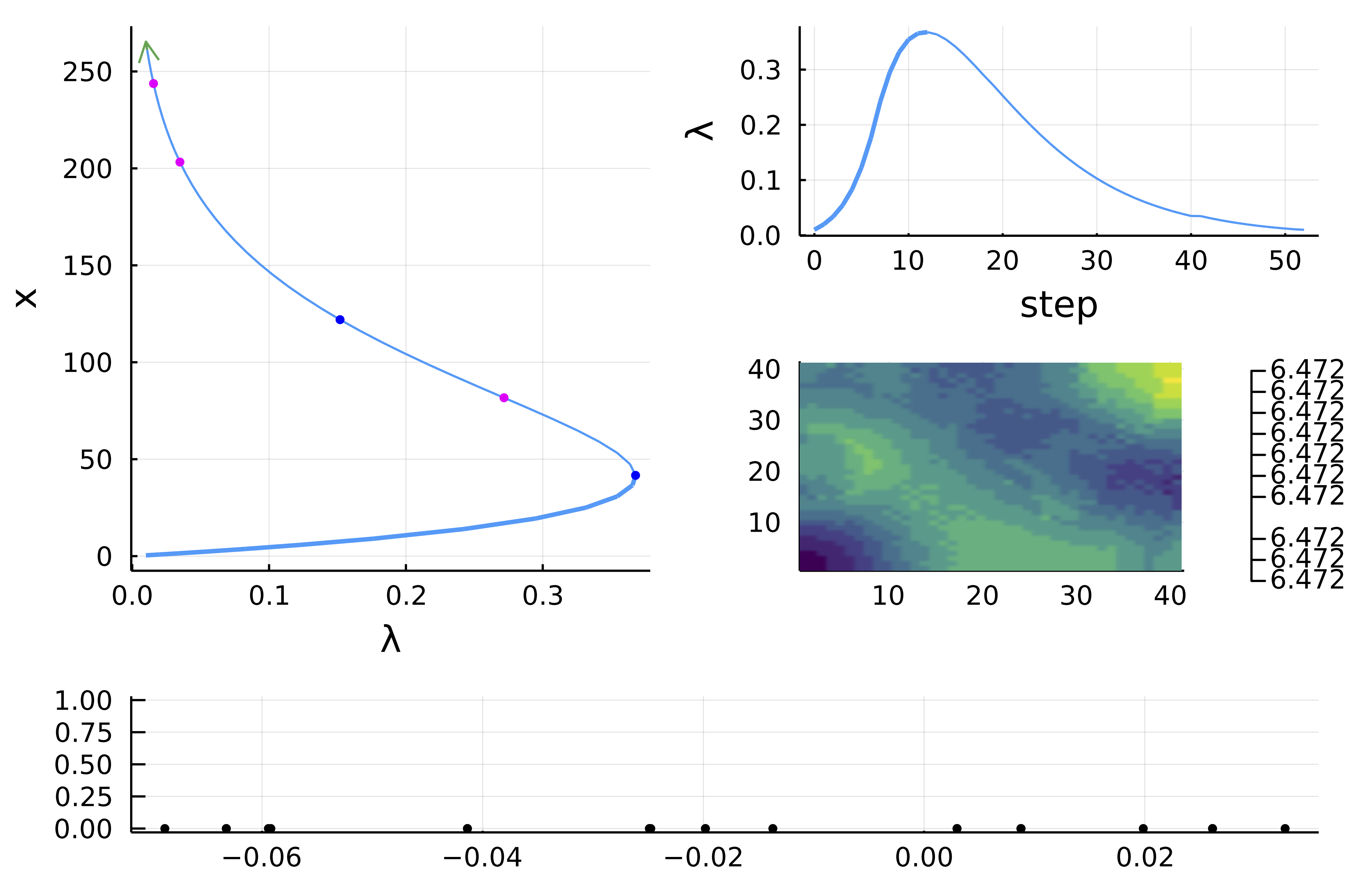                                                                    step =  55

Computation of the first branches

Let us now compute the first branches from the bifurcation points. We start with the one with 1d kernel:

br1 = continuation(br, 3,
	setproperties(opts; ds = 0.005, dsmax = 0.05, max_steps = 140, detect_bifurcation = 3);
	verbosity = 3, plot = true, nev = 10,
	usedeflation = true,
	callback_newton = BifurcationKit.cbMaxNorm(100),
	)

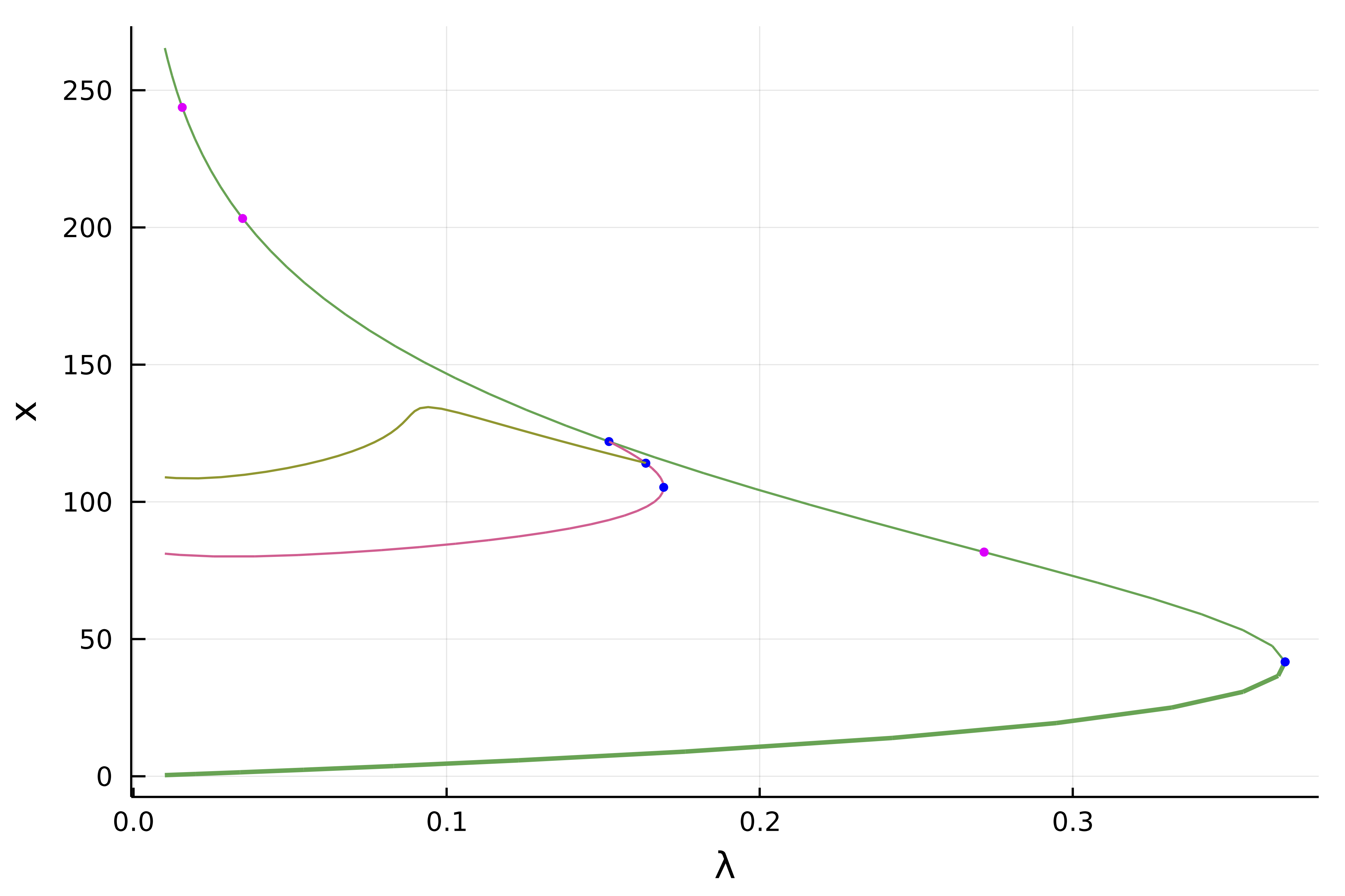
We also compute the branch from the first bifurcation point on this branch br1:

br2 = continuation(br1, 3,
	setproperties(opts;ds = 0.005, dsmax = 0.05, max_steps = 140, detect_bifurcation = 3);
	verbosity = 0, plot = true, nev = 10,
	usedeflation = true,
	callback_newton = BifurcationKit.cbMaxNorm(100),
	)

plot(br, br1, br2)

We get:

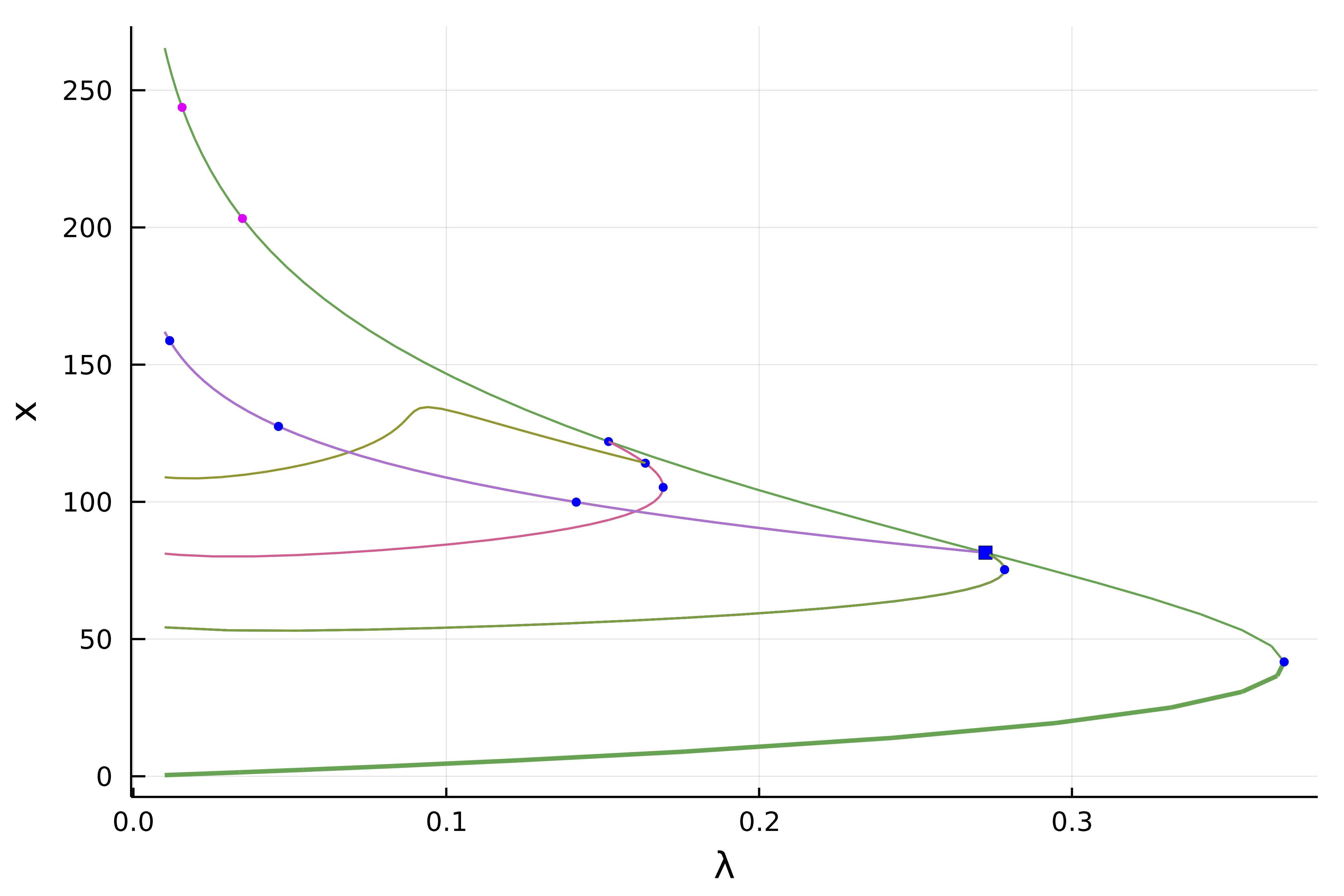
Finally, we compute the branches from the 2d bifurcation point:

br3 = continuation(br, 2,
	setproperties(opts; ds = 0.005, dsmax = 0.05, max_steps = 140, detect_bifurcation = 0);
	verbosity = 0, plot = true,
	usedeflation = true,
	verbosedeflation = false,
	callback_newton = BifurcationKit.cbMaxNorm(100),
	)

plot(br, br1, br2, br3...)