🟢 1d Kuramoto–Sivashinsky Equation

• 🟢 1d Kuramoto–Sivashinsky Equation
• • Computation of the bifurcation diagram

We study the 1d Kuramoto–Sivashinsky equation with Dirichlet boundary conditions:

\[\left(2 u u'+ u''\right)+2\lambda u^{(4)}=0,\ u(0)=u(\pi)=0.\]

We discretize the problem by using $u(x)=\sum_{k=1}^{\infty} u_{k} \sin (k x)$ which gives

\[\left(2\lambda k^4-k^2\right) u_{k}+\frac{k}{2}\left(\sum_{l=1}^{\infty} u_{k+l} u_{k}-\frac{1}{2} \sum_{l+m=k} u_{l} u_{m}\right)=0.\]

This is a good example for the use of automatic bifurcation diagram as we shall see. Let us first encode our problem

using Revise, LinearAlgebra, Plots
using Parameters, Setfield, ForwardDiff
using BifurcationKit
const  BK = BifurcationKit

# we use this library for plotting
using ApproxFun

function generateLinear(n)
	Δ = [-k^2 for k = 1:n]
	return Δ, Δ.^2
end

function Fks1d(a, p)
	@unpack Δ, Δ2, λ, N = p
	out = (2λ) .* (Δ2 .* a)
	out .+= (Δ .* a)
	for l=1:N
		for m=1:N
			if 0 < l+m <= N
				out[l+m] += l*a[l]*a[m]
			end
			if 0 < m-l <= N
				out[m-l] += l*a[l]*a[m]
			end

			if 0 < -(m-l) <= N
				out[l-m] -= l*a[l]*a[m]
			end
		end
	end

	out .*= -1
	return out
end

Having defined the model, we chose parameters:

N = 50
Δ, Δ2 = generateLinear(N)
par_ks = (Δ = Δ, Δ2 = Δ2, λ = 0.75, N = N)

# we define a Bifurcation Problem
prob = BifurcationProblem(Fks1d, zeros(N), par_ks, (@lens _.λ),
  record_from_solution = (x, p) -> (s = sum(x), u2 = x[3], nrm = norm(x)),
  plot_solution = (x, p; kwargs...) -> plot!(Fun(SinSpace(), x) ; kwargs...),)

and continuation options

optn = NewtonPar(tol = 1e-9, max_iterations = 15)
optc = ContinuationPar(p_min = 1/150., p_max = 1., max_steps = 700, newton_options = optn,
dsmax = 0.01, dsmin = 1e-4, ds = -0.001, nev = N, n_inversion = 8,
max_bisection_steps = 30, dsmin_bisection = 1e-10, plot_every_step = 50)

kwargscont = (verbosity = 2, plot = true, normC = norm)

Computation of the bifurcation diagram

# function to adapt continuation option to recursion level
function optrec(x, p, l; opt = optc)
	level = l
	if level <= 2
		return setproperties(opt;  dsmax = 0.005, max_steps = 2000, detect_loop = true, n_inversion = 6)
	else
		return setproperties(opt;  dsmax = 0.005, max_steps = 2000, detect_loop = true, n_inversion = 6)
	end
end

# we now compute the bifurcation diagram
# that is the connected component of (0,0)
diagram = @time bifurcationdiagram(prob, PALC(), 4, optrec;
		kwargscont..., verbosity = 0,
		)

Plotting the result can be done using

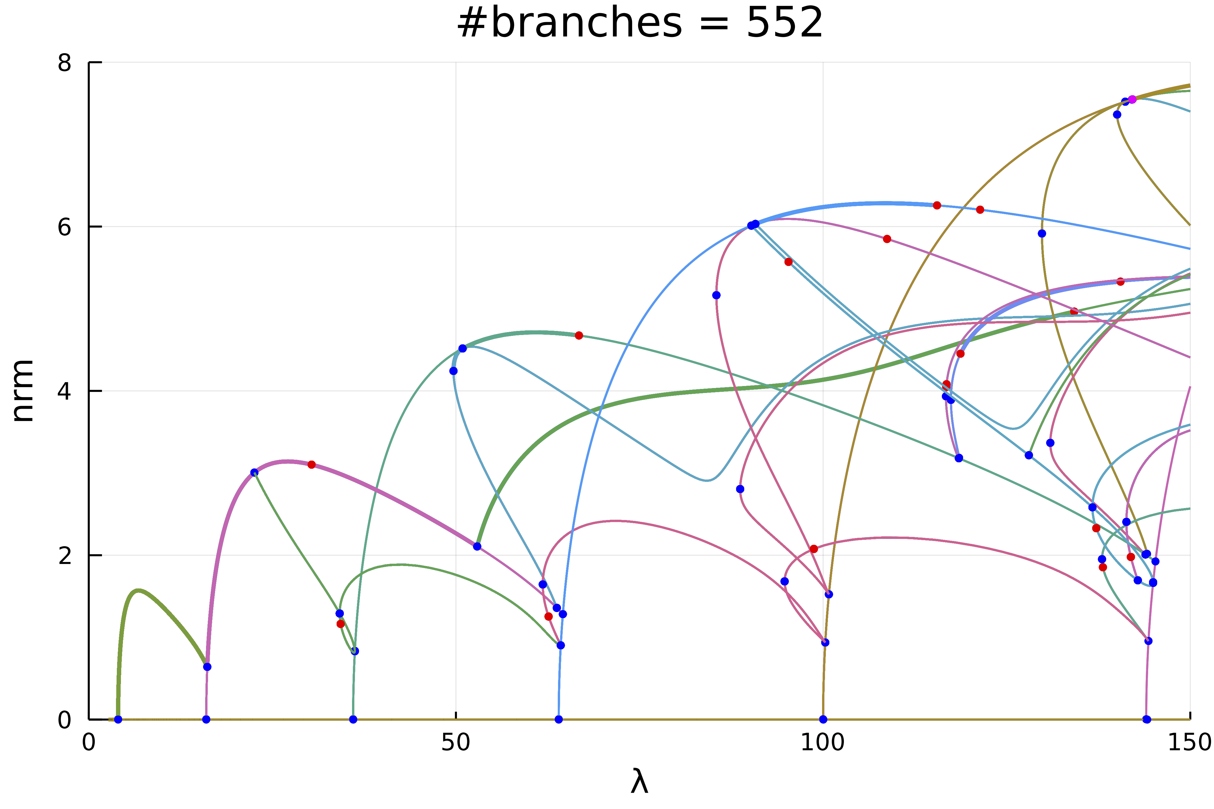
plot(diagram; code = (), plotfold = false,  markersize = 3, putspecialptlegend = false,
	 plotcirclesbif = true, applytoX = x->2/x, vars = (:param, :nrm),
	 xlim = (0,150), ylim=(0,8))
title!("#branches = $(size(diagram))")