🟢 Plane

• 🟢 Plane

In this tutorial, we show how to cover a plane as solution of

\[F(u) := u_3 = 0\]

We use this model as a mean to introduce the basics of MultiParamContinuation.jl.

It is easy to encode the manifold as follows

using CairoMakie, MultiParamContinuationconst MPC = MultiParamContinuationF(u,p) = [u[3]]prob = ManifoldProblem(F, [.0,0.,0.], nothing;                        # we pass a function to provide the tangent space                        # with an analytical formula                        get_tangent = (u,p) -> [1 0; 0 1; 0 0],                        # restrict computations to hypercube                        finalize_solution = Cube(0.5)                        )

2-d Manifold Problem
    ├─ n = 3
    └─ m = 1

show(prob)

2-d Manifold Problem
    ├─ n = 3
    └─ m = 1

We now compute a covering of the manifold.

S = MPC.continuation(prob,            Henderson(np0 = 4),            CoveringPar(max_charts = 20000,                    max_steps = 100,                    verbose = 0,                    R0 = .1,                    ))show(S)

Surface 2-d
   ├─ # charts = 101
   └─ problem =
          2-d Manifold Problem
              ├─ n = 3
              └─ m = 1

You plot the result as follows

MPC.plotd(S;    draw_tangent = true,    plot_center = true,    draw_edges = true,    )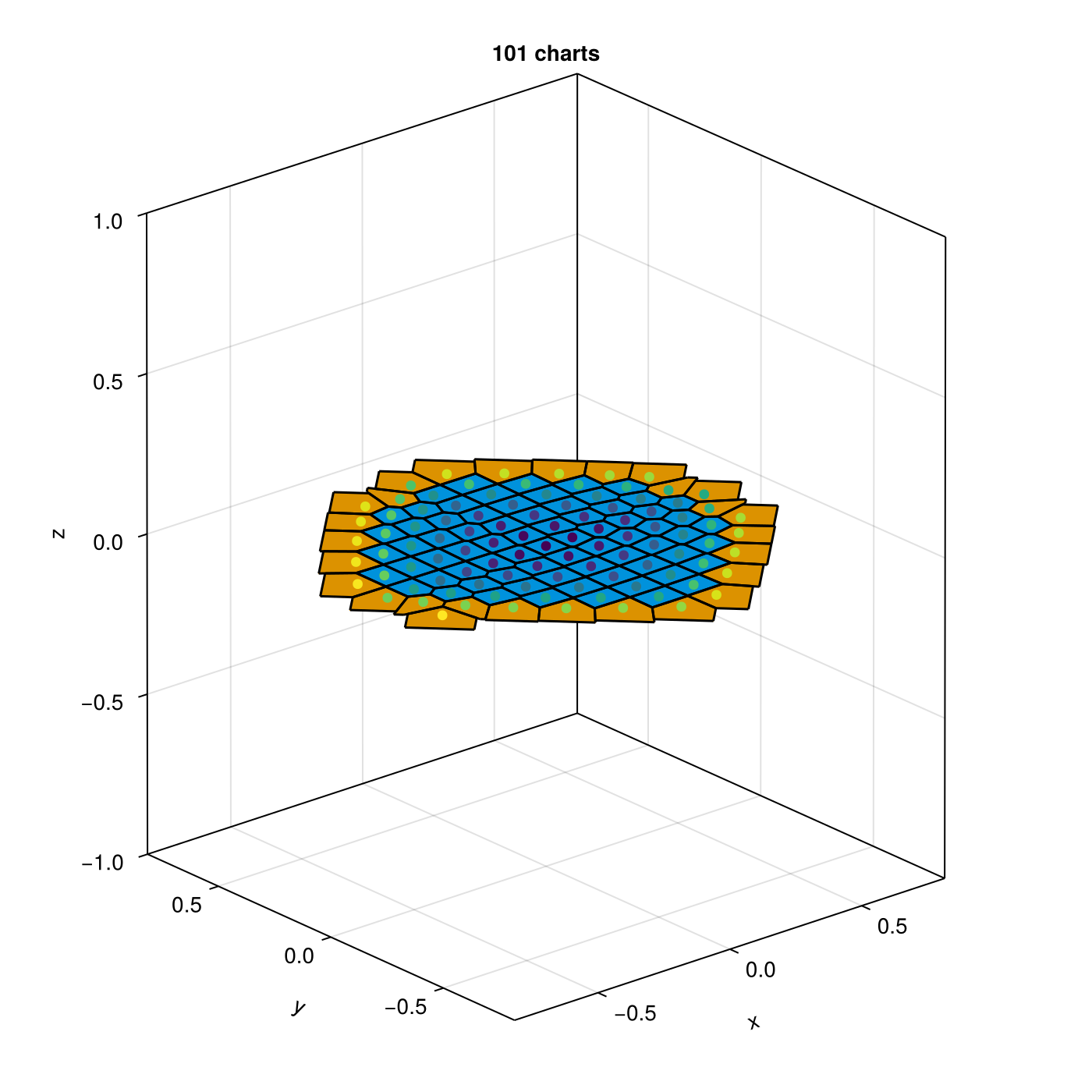

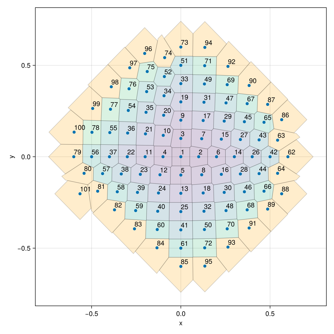
It is sometimes useful to have access to more information, and for example plot in 2d:

MPC.plot2d(S;    draw_circle = true,    plot_center = true,    put_ids = true,    ind_plot = [1,2])